Navigation : Home : FoveaPro : FoveaPro Tutorial : Part 21
Image Analysis Cookbook 6.0: Part 21
6.E. Measuring features
Choosing the appropriate measurement is important. Knowing as much as possible about the application is important in choosing the measurements that are meaningful. Feature measurements can be grouped into four categories:
Size (area, length, breadth, perimeter, etc.) : Most of these measures are easily understood. The perimeter is measured using an exceptionally accurate super-resolution method. The convex area and perimeter are based on a convex hull (also called a rubber-band or taut string bounds).
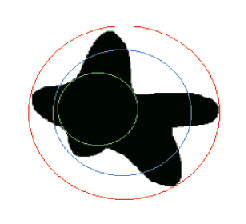
An irregular feature with the maximum distance (“length”), convex bounds (used for convex area
and convex perimeter), circumscribed circle, inscribed circle and equivalent area circle shown.
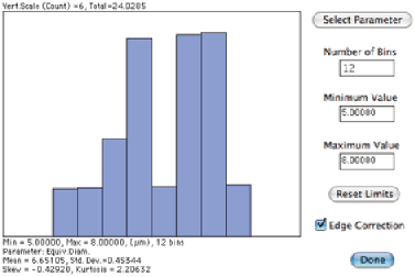
In many cases, the size distribution of features is based on the area, the equivalent circular diameter, or the maximum caliper dimension (length). The example shows the length of rice grains.
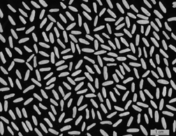
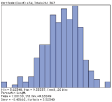
Original Rice2 image and distribution of lengths of grains
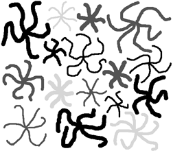
The length or breadth of a curved feature is determined as shown in Section 5.E.1. using the skeleton and the Euclidean distance map. The example shows several irregular star-shaped features that are classified and color-coded by the number of arms, the width of the arms, and the length of the arms. By assigning values proportional to each of these measurements in the R, G and B channels, the pairs of features that share all three properties are given the same color and visually identified.
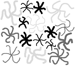
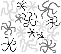
The Stars2 image with features shaded according to the length and breadth of external branches.
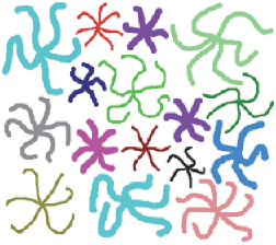
Features coded by the number of branches, and with values for all three parameters in RGB channels.
Shape (topology, dimensionless ratios, fractal dimension) : Shape is one of the most difficult properties to describe either verbally or numerically. Ratios of size parameters are convenient but not specific, and are given arbitrary names that are neither unique nor consistent. Topology, using the feature skeleton, captures one important aspect of shape as shown above. Fractal dimension corresponds to the boundary irregularity or “roughness”.
The example shows a regression plot of feature shape (form factor, defined as 4πArea / Perimeter 2 ) vs. size (equivalent diameter) for the Dendrites image shown above. The strong correlation results because the small features are intersections with the branches of the dendrites (which tend to be round) while the large features are intersections with the trees (which are more irregular). Fracture, agglomeration, etc. all tend to produce variations of size with shape.
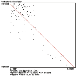
Scatterplot of size vs. shape for the features in the Dendrite image
The fractal dimension of Euclidean shapes (circles, squares, etc.) is 1. As the irregularity (“roughness”) of the feature boundary increases, so does the dimension.
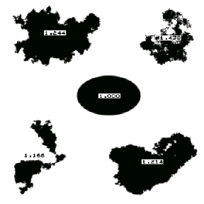
Features in the FShapes image labeled with their fractal dimension values.
Intensity (density, color) : These require calibration as discussed above. True spectral information cannot be obtained from a tristimulus camera or scanner, but the hue values for features often correspond to their visual “color.” The example shows the measurement of features (after thresholding, watershed segmentation, and masking of the original image) and a scatterplot of hue vs. intensity that groups the various candies.
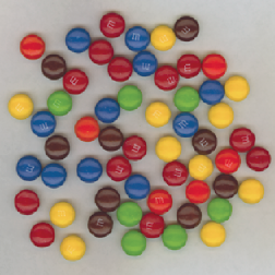
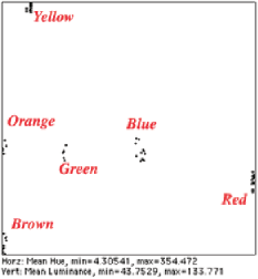
Original MandM image, and a labeled plot showing the hue and intensity values of the various candies
Location (absolute coordinates or distances from other objects) : The coordinate position of features is measured from the upper left corner of the image, in whatever calibrated units have been established. This can be important for specific cases such as locating spots on scanned gels, but in most cases it is the position of features relative to other features present in the image that is most interesting. Neighbor relationships can be important for understanding structure.
There are several different points that can be chosen for the location of a feature, and distances can be measured from centroid to centroid or edge to edge. Spatial clustering or self avoidance can be measured by comparing the mean nearest neighbor distance to 0.5 • sqrt (Area / Number). Adjacent neighbors can be counted. Note that the definition of “adjacent” in this routine is features that are separated by a single-pixel-wide four-connected line. In most cases the easiest way to produce such an image is to skeletonize the background between the features (or the cell walls or grain boundaries in a structure). The skeleton is an 8-connected line (pixels touch any of their eight neighbors), which can be converted to a 4-connected line (pixels touch only their four edge-sharing neighbors) that separates features by selecting Morphology –>Thicken Skeleton . Then invert the image so that the lines are white and the features black, and count adjacent neighbors.
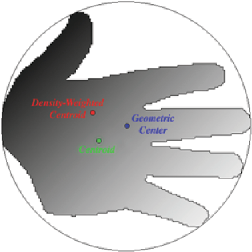
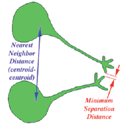
Definitions for location and neighbor distances
The examples show the measurement of clustering and adjacent feature counts. Section 5.E.1 showed the measurement of individual feature distances from a boundary.
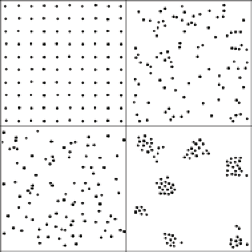
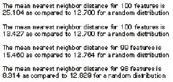
Clusters image and the measurement of clustering results for the four regions
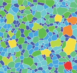
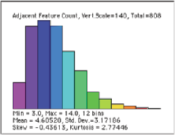
Gr_Steel image with the grains color-coded by number of adjacent neighbors and a distribution plot
6.F. Data analysis and feature recognition
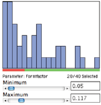
Measurement data can be used for feature classification by establishing a recipe with limits on various measurement parameters. This is equivalent to carrying out a series of feature selection measurements to isolate each set of objects. In the first example, the IP•Measure Features–>Select Features routine is used to select the characters in the script fonts based on their formfactor. The selected features are given the foreground (pen) color and the others are given the background (eraser) color.
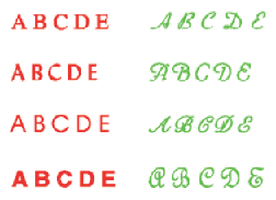
The Fonts image after selecting features based on formfactor
A recipe file contains the parameter names and limits and optionally the color values used for labeling. The example shown is used to identify (and color code) the letters A through E, in different fonts and sizes. IP•Measure Features–>Color by Value and –>Label Features allow selection of a class parameter when a recipe file has been defined ( IP•Utilities–>Select Recipe File ), and the class is included in the output from the IP•Measure Features–>Measure All Features routine.
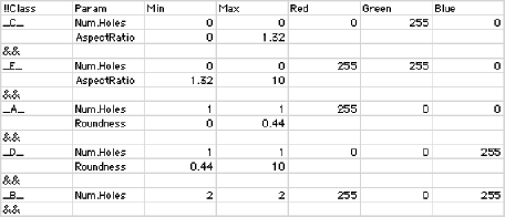
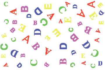
A recipe file used to automatically color code the letters in the A2E image