Navigation : Home : FoveaPro : FoveaPro Tutorial : Part 19
Image Analysis Cookbook 6.0: Part 19
6. Measurements
6.A. Calibration
6.A.1. Calibrating image dimensions
Establishing a calibration that can be used by the various measurement routines is typically done by acquiring an image of a stage micrometer or some standard object. A micron marker on an scanned image can also be used. The procedure in the IP•Measure Global–>Calibrate Magnification routine is to mark two points on the image and enter the distance between them (and select the units). Calibrations can be saved to disk by name (e.g., one for each objective lens on a light microscope) and recalled as needed.
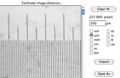
The IP•Measure Global–>Calibrate Magnification dialog
Note that the magnification calibration is not tied to a specific image, but rather is a system constant that stays in effect for all measurements until it is changed.
6.A.2. Calibrating density/greyscale values
Constructing a curve relating pixel value (0..255) to density, or any other parameter, requires standards. These are readily available at macro scales but harder to make or obtain for microscopes. Recalibration is needed often because of variation in line voltages, lamp aging, optical variations, camera instabilities, etc. It is also important to turn off any automatic gain adjustments in the camera or scanner. The procedure is to measure the average brightness of uniform known regions and then enter the values into the IP•Measure Global–>Calibrate Density routine. The resulting curve can be stored on disk and recalled as appropriate. It is also possible to construct calibration curves of pixel value vs. distance to use with EDM-based measurements.
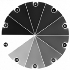
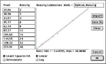
The DenWedge image and its calibration curve
6.B. Measurement of principal stereological parameters
Relationships between three-dimensional structure and two-dimensional images provide methods to correctly measure metric properties such as volume fraction, surface area, length, etc., as well as topological properties such as number and connectivity. Modern stereology emphasizes the best ways to perform sampling and sectioning to avoid bias.
6.B.1. Volume Fraction
The volume fraction of a region, phase or structure in a 3D volume is measured by the area fraction shown on a random plane section (or better, averaged over many such sections). The Measure Global –> Area Fraction plug-in reports (and writes to the log file if logging is turned on) the percent of the image that is not white background. If an area of the image has been selected with the marquee, lasso or wand selection tools, the reported value is the fraction of the selection area that is not white. In most cases the image being measured will be a binary (black and white) image as a consequence of thresholding and perhaps the application of Boolean logic, and the measured area is defined by the black pixels, but the plug-in is equally applicable to images in which features of any grey scale or color value are present, on a white background. The area fraction value measured with this plug-in is identical to the result that could be obtained by summing the contents of the histogram for all values other than white (255).
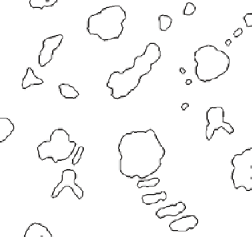
As an example, in the image Drawing (shown), thresholding the grey cells produces a binary image in which the area fraction is reported as 16.93%
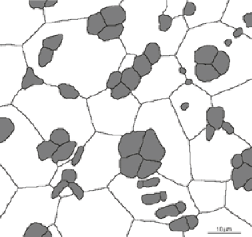
Original Drawing image Thresholded grey cells
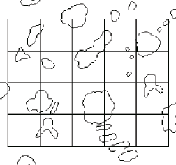
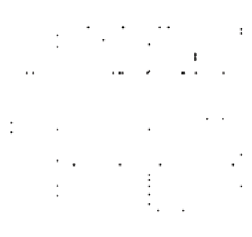
Another way to measure volume fraction (or area fraction) is to use a grid of widely spaced points (ideally separated far enough that rarely do two points in the grid fall on top of the same feature in the image) and count the fraction of the points that lie on the structure of interest. The advantage of the technique is that it allows a direct estimate of the precision of the volume fraction measurement, because the statistics of counting are such that the standard deviation in the number counted is just the square root of the number. In other words, if a grid with 100 points (10 x 10 array) is used and one third of them (33) fall on features that constitute the structure of interest, then the result is 33 ± 6 (approximately the square root of 33). If it is desired to obtain an overall measurement precision of 5%, then additional fields of view should be similarly measured, and it can be expected that about 11 more fields will be needed, because a total of 12 fields times about 33 hits per field would be 400 points counted, and the square root of 400 is 20, or 5%. Designing an experiment to collect the required number of fields of view so that they adequately represent a real specimen is an important consideration, and usually requires sampling a few images to get a rough idea of the magnitude of the values of interest.
To apply a grid to an image, an efficient procedure is to duplicate the image ( Image–>Duplicate ) and then erase it ( Select–>All and Edit–>Clear , assuming the background color has been set to white). Layers can also be used. A Photoshop action implementing this sequence and assigning it to a function key is easily set up. If many images of the same size are to be processed, the image of the grid can simply be saved to disk for re-use. Generating a grid of points or lines is selected under the Points and Lines menu. In the examples shown below, the points have been dilated for better visibility.
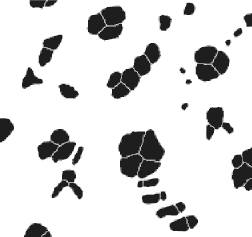
In this example, the volume fraction of the lung that is air space is wanted. But the lung tissue does not cover the entire field of view, so two measurements are needed, to measure the total lung area and the tissue area. The original image was leveled and thresholded to produce a binary representation of the tissue, and then a grid with 90 points was generated. Applying a Boolean AND to combine the grid with the binary image of the tissue and counting the number of points reports 29 hits.
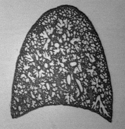
Original RatLung image Binary representation
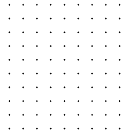
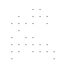
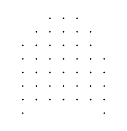
Generated 90 point grid Grid ANDed with binary
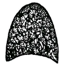
Next, the binary image of the tissue has its holes filled in ( Morphology–>Fill Holes ) to produce an image of the total lung cross section. This is also combined with the grid using a Boolean AND and the hits counted (44). The area fraction of the cross section that was originally air space is thus (44 – 29) / 44, or 34 percent. To properly estimate the volume fraction of the lung, multiple sections should be taken at different positions in the organ, and the counts for net tissue area and full cross section area summed individually before being used in the calculation of the percentage.
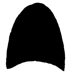
Binary with holes filled Grid ANDed with filled image
A manual procedure using grids with visual recognition of the structure is to superimpose the grid directly onto the image (usually with a contrasting or colored pen color), select a pencil of convenient size and unique color, and manually mark the points that are to be counted. The IP•Measure Features–>Count plug-in reports the number of separate marks in the current pen color, and the resulting image can be saved as a record of the procedure if desired.
6.B.2. Surface Area
The surface area per unit volume of the boundaries between regions in the 3D volume (which may either be identical phase regions, such as the grains in a metal separated by grain boundaries, or dissimilar regions, such as the surface of membranes that surround and separate organelles from the rest of the cytoplasm of a cell) can be measured stereologically. These 3D surfaces are revealed on two-dimensional section planes as lines. If the lines are broad, as for example would be produced by etching grain boundaries for visibility, or sectioning through membranes at a shallow angle, the resulting image can be skeletonized to reduce the lines to ideal single-pixel width. Thresholding of original grey scale or color images, and perhaps other processing, is typically used to obtain an image in which the boundaries whose surface area per unit volume is to be measured are delineated by a line of black pixels on a white background.
There are two principal relationships used to measure the surface area per unit volume. One is based on the length of the lines of intersection between the surfaces of interest and the sampling plane that is imaged. The other draws line grids on the image and counts the intersections between the grid lines and the lines that represent the trace of the surface on the plane of examination. The latter method may be preferred because it is a counting rather than a measurement operation. Also, it is possible to generate specific kinds of grids (e.g., circles, cycloids, random lines) that can be used with specific kinds of section orientations to obtain isotropic sampling of structures that have a preferred orientation. It must be assumed for purposes of making this measurement that either the surfaces of interest are isotropically oriented in 3D space, or that the section planes that have been imaged are oriented in such a way that isotropic sampling is obtained. One such technique is to cut so-called “vertical” sections and then draw cycloids on the surface.
Given a suitably obtained and processed image (or set of images) the surface area per unit volume can be measured by Sv = (4/π) • Length of line / Area of image. The IP•Measure Global –> Total Line Length plug-in reports the total length of lines present in the image, as well as the total area of the image or selection. This method can be used for either a full image area or for any rectangular region defined by the marquee selection tool. However, if applied to a non-rectangular selection region it actually measures the area and contents of the bounding rectangle that fits around the arbitrary-shaped selection. Inverting the selection and erasing exterior lines can be used to deal with any problems this might cause.
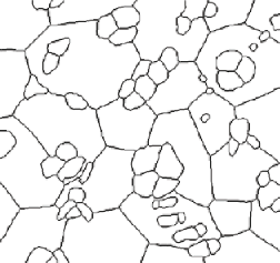
To illustrate this procedure, the test image ( Drawing ) shown above represents a structure with two type of grains or cells, grey and white. By application of morphological and Boolean logic any of the three types of surfaces can be isolated (the grey-grey cell boundaries, the grey-white cell boundaries, and the white-white cell boundaries). As an example, by thresholding the grey cells, performing a closing, selecting the outlines, and skeletonizing, the boundaries between the grey and white cells are delineated as shown.
Closing to eliminate grey-grey boundaries Skeletonized outlines
Measuring the total length of the skeleton lines reports values of 547.08 µm for the line length and 5453.6 µm 2 for the image area, which by the equation above produces a value of 0.1277 µm –1 for the surface area per unit volume. Note that the measurement of volume fraction above did not depend on the calibration of the image magnification, since the units cancel out, but the measurement of surface area does require that the calibration be performed beforehand.
Grid lines superimposed on the outlines Intersection points produced by ANDing
For comparison, the second measurement procedure using a grid of lines is also shown. A rectangular line grid was used, but the same method would apply to circles, cycloids, or random lines. ANDing the grid with the outlines and counting the number of intersections (which are shown dilated in the example for visibility) produced 45(±6.7) counts with a grid line length of 680.49 µm. Using the equation above, the resulting value for surface area per unit volume is 0.1323(±0.0197) µm –1 , in good agreement with the line length method above.
6.B.3. Line length
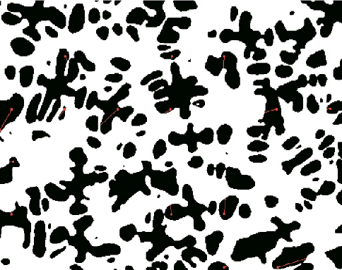
The length of lines in a 3D volume is calculated from the number of intersections that they make with the section plane. In the structure shown in the example image, the triple lines where three cells or grains meet are one such linear structure. These can be isolated by thresholding all of the cell boundaries in the image, skeletonizing, and selecting just the nodes (points in the skeleton with more than two neighboring pixels - these are shown dilated for visibility in the illustration). Counting these reports 145 intersections of the triple lines with the image, whose area are noted above is 5453.6 µm 2 . The line length per unit volume is 2 • Number of Intersections / Area, and thus is calculated as 0.0532 µm – 2 . Obviously, this measurement also requires the prior calibration of the image. Boolean logic combined with morphological dilation of the phase regions can be used to select triple lines that lie at the junctions of the various phases present.
Skeletonized boundaries Nodes (dilated for visibility)
 Another procedure often used to measure line lengths in volumes applies to transmission images through thin sections. The linear structures appear in such images as lines, which can be thresholded and skeletonized. Drawing a grid of lines on the image represents a set of surfaces extending down through the thickness of the section (whose thickness must be independently known). As usual, the grid lines must be made isotropic in 3D by appropriate selection of section orientation and choice of grid lines, if the sample is not itself isotropic in structure; this is sometimes done by using vertical sectioning and cycloids, or random sectioning and circles. In either case, ANDing the grid lines with the skeleton of the linear structure and counting the intersections produces a number of counts. This is used in the same calculation as above, namely length per unit volume equals 2 • Number of Intersections / Area, but now the area is the area of the surfaces that extend from the grid lines through the imaged section. This is just the thickness of the section times the length of the grid lines.
6.B.4. Intercept lengths
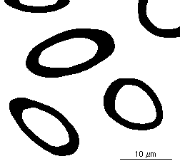
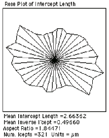
The mean intercept length through a structure can be measured by drawing lines and ANDing them with the binary image of the structure, followed by measuring the length. This is most efficiently done by the IP•Measure Global–>Intercepts plug-in, which automatically generates a grid of parallel lines with orientations that vary systematically in ten degree steps, and reports the mean value (3.574 µm in the example shown) as well as showing the rose plot to reveal any anisotropy in the structure.
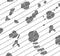
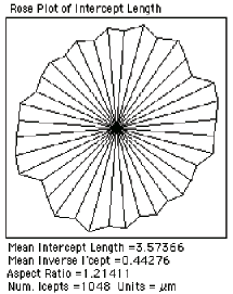
Parallel line grid overlaid on thresholded cells Intercept length plot as a function of orientation
This routine also reports the mean inverse intercept length, which is important for measuring the true three-dimensional thickness of a layer structure cut at random angles by the section plane. The true 3D thickness is (3/2) • 1/Mean Inverse Intercept Length. For example, in the image shown ( Thickness ), the mean inverse intercept is reported as 0.4966 µm –1 . That produces a calculated true thickness value for the sheaths of 3.02 µm.
Thresholded image of sections through layers Measured intercept data
6.B.5. Number per unit volume
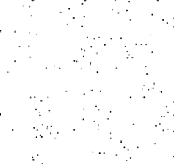
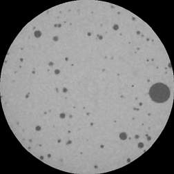
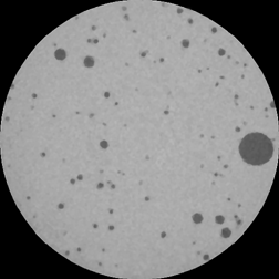
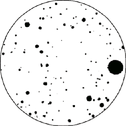
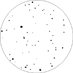
A single image does not directly reveal the number of objects per unit volume. A section plane is more likely to intersect large features than small ones. Counting the number of features seen per unit area is only indirectly related to the number per unit volume, but in some instances the desired information can be obtained. In the example shown ( Whip ), an image of bubbles in a whipped food product, it is reasonable to assume that all of the bubbles are the same size (created by the same gas pressure), and the different sizes of the circular intersections represent cutting through a sphere at different latitudes. It is easy to measure the size distribution, as shown, but not very useful. There are procedures for “sphere unfolding” that can use the size distribution of the circles with the assumption of a spherical 3D shape to calculate the size distribution of spheres that must have been present for random sectioning to generate the observed result, but they are notoriously sensitive to counting statistics and to any slight variations in shape of the structure.
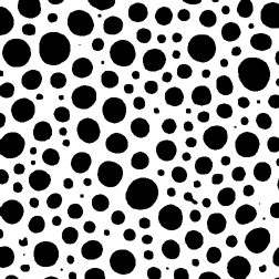
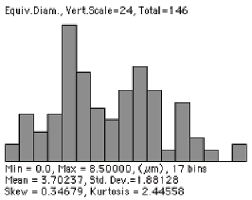
Thresholded bubbles Measured 2D feature sizes
But for random sections through a unit sphere, the mean intersection circle has a diameter 2/3 that of the sphere. So for the measured mean circular diameter of 3.702 µm, the corresponding mean sphere diameter is estimated to be 5.56 µm. There are 146 features (corrected for edge-touching as discussed in Section 6.D) in an image area of 5053 µm 2 . The relationship between number per unit volume (N V ) and number per unit area (N A ) is N V = N A / D mean , so the calculated number per unit volume is 5.2 • 10 –3 per µm 3 . Since the volume fraction (measured by the area fraction as described above) is 40.22%, the mean volume of each sphere can be calculated (77.32 µm 3 , which corresponds to a diameter of 5.29 µm and is in reasonable agreement with the original assumption). This method is applicable to any shape of particle, provided that a meaningful estimate of the mean diameter can be obtained.
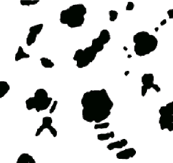
6.B.6. The Disector
A modern stereological technique for directly counting the number of features per unit volume requires imaging two section planes a known distance apart. This distance must be smaller than the size of any feature of interest, so that by comparing the two images it is possible to know what happens in the volume between the two planes. The images are aligned (this is usually conveniently done by placing them in layers) and features are counted that intersect either one of the two section planes (and thus appear in either one of the two images) but not in both. In the example shown ( Musketrs ), the two images are sequential CT slices, and confocal microscope optical sections are also convenient because they are automatically aligned. Each image is thresholded to show the features of interest (the holes). To automatically count the holes that are distinct between the two, the IP•Math–>Select Features by 2nd plug-in is used to combine copies of image 1 with image 2 as shown in section 5.C.2 and vice versa. ORing these two images together marks all of the features that cross one or the other of the image planes, but not both. These represent the tops and bottoms of the holes, so the number per unit volume is just half of the count divided by the volume (the product of the area times the distance between image planes).
Two sequential sections through a candy bar (CT slice images)
There are 65 features that are present in either image and not matched in the other image. The area of the section is 1.54 cm 2 , and the distance between them is 6.3µm. The number per unit volume is then calculated as (Number of Counts / 2) / Volume, or 32.5 / 9.7 mm 3 , giving a net result of 3.35 holes per mm 3 . Combined with the total volume fraction of holes (determined from the area fraction as described above), the average volume per hole is 0.0018 mm 3 . This result is completely independent of any shape assumption, and is valid for features of varying shape, even if the shape varies with size. Furthermore, since the disector is a volume probe of the sample, it is not necessary to use special sectioning techniques to obtain isotopic orientations or special alignments.
Thresholded binary image of one slice Features in one but not both sections, for counting
The disector can also be used to calculate the connectivity of network structures. In that case, three types of events must be counted by comparing the features in the two sections. As before, features that simply extend through both section planes without any change in topology (although of course they may change in shape or size) are ignored. Features that end between the two sections (and thus appear in one image but not the other) are counted as T++ events. Ones that contain holes in one image that have filled in in the other are counted as T–– events. Features that split or branch between the two planes, so that a single feature in one image becomes two in the other, are counted as T+– events. The calculation is then Net Tangent Count equals the sum of the T++ and T–– counts minus the T+– counts. From this, the connectivity of the structure (the number of cuts per unit volume that can be made without disconnecting it, also known as the Euler number for the network) is given by the relationship N V – C V = (1/2) • Net Tangent Count / Volume. In most cases for a complex network structure, N V , the number of objects per unit volume, is 1 and the connectivity C V is determined primarily by the number of branching events in the volume between the two images. If appropriate, viewing the images in layers with partial transparency can be used with manual marking of the various types of events with different colors for counting.
6.B.7. Point sampled intercepts
By combining the disector method of determining the number of features per unit volume, which is not sensitive to shape, with a grid-based measurement method, it is possible to determine even more about the sizes of features present in a structure. The method of point-sampled intercepts places a grid of points onto the binary image. Each point that hits a feature in the image is used to generate a line whose length to the edge of the feature is measured. By using the length of each line to estimate the volume of the feature as (4π/3) • r 3 , a mean value of the volumes can be obtained. However, this is the volume-weighted mean volume, not the more familiar number-weighted mean. That means that large features are more likely to be measured, because the points in the grid are more likely to fall on a large feature than on a small one.
But the usual number-weighted mean value of volume can also be determined by combining the volume fraction (measured in one of the ways described above) and the number per unit volume (determined using the disector). And the difference between the volume-weighted mean and the number-weighted mean is just the variance of the distribution of volumes of the particles, so the standard deviation of that distribution (the square root of the variance) can be determined, again without any sensitivity to feature shape.
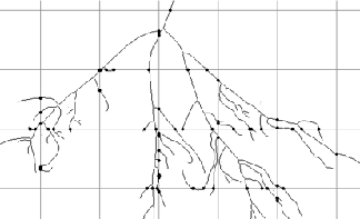
Dendrite image, thresholded with a superimposed grid of point-sampled lines (colored for visibility)
The procedure for applying this method is executed by the IP•Lines and Points–>Point Sampled Intercept plug-in, which generates a regular grid of points with the user-specified spacing. The angles of the generated line segments may be either uniformly distributed or sine-weighted (for use with vertical section images). In the example shown, this reports a mean cubed radius of 7.965 µm 3 . Multiplying by (4π/3) gives a volume-weighted mean volume of 33.36 µm 3 .
6.B.8. Other stereological methods
The plug-ins include routines that implement specific stereological techniques such as tangent counts, measurement of ASTM grain size in images of metal grains, and characterization of feature clustering or self-avoidance. These techniques and the examples shown do not exhaust the variety of measurements that stereology can provide as a meaningful description of the three-dimensional structure of solids based on the two-dimensional images that are captured for examination. Books on stereology, such as Russ & Dehoff, Practical Stereology, 2nd edition, 2002, Plenum Press, provide descriptions and examples of both the classical methods and the so-called “new” or “unbiased” techniques that depend heavily on proper sectioning procedures and are not dependent upon any assumptions about shape or isotropy. However, most of these methods use the same plug-in procedures already described, relying on the generation of an appropriate grid, its Boolean combination with a binary representation of the structure, and counting (or in some cases measuring) the result.