Navigation : Home : FoveaPro : FoveaPro Tutorial : Part 20
Image Analysis Cookbook 6.0: Part 20
6.C. Intensity and Color
Profiles of intensity, calibrated density, or color information often provide efficient ways to extract data for analysis and can simplify measurement of dimension. Radial plots from the center of an image or region, plots along arbitrary lines, or averaged intensity values across horizontal regions are all saved in disk files for analysis in a spreadsheet. If an intensity calibration curve has been created or loaded, the calibrated values are shown. Spatial calibration is used to convert the pixel distances to real units.
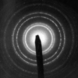
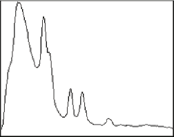
Original E_Diff image and a plot showing the averaged radial intensity
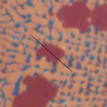
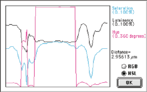
Original Alloy image and a line profile showing the color information
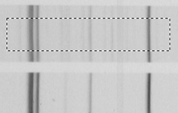
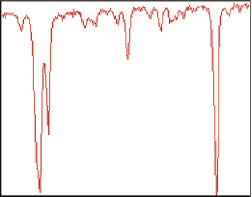
Debye image (fragment) with the averaged intensity profile of the region marked
Feature measurement parameters include brightness, calibrated density, and color information for the pixels within them. These data are saved in disk files, or can be used to label the display. Note that in the example shown, a calibration standard is scanned along with the gel and used to calibrate the density measurements.
Measurement of the optical density in the GelSep image, calibrated using the built-in standards
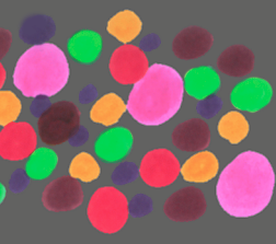
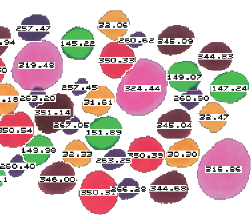
Original ColrDots image (fragment) and the features labeled with their hue, which is
an angle from 0 (red) through green (120), blue (240) and so on to 360 degrees. The image was
thresholded and watershed segmented to create a mask used to isolate the features for measurement.
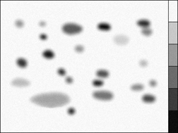
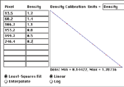
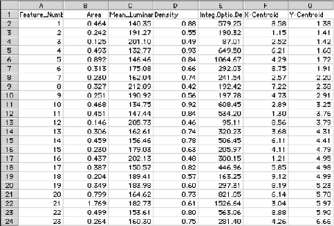
The integrated optical density (IOD) provides a tool for counting features in three-dimensional clusters. Create a logarithmic (Beer’s Law) calibration curve using the background intensity (measured as 220 on a representative area of the image shown) for zero optical density, and measure the IOD of each cluster. The ratio of the IOD for a cluster to that for a single particle estimates the number of particles in the cluster.
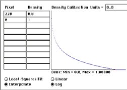
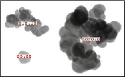
Calibration curve and IOD measurements for a few features in the CarBlac2 image.
The procedure estimates 12 and 87 particles in the two clusters, respectively.
6.D. Counting features
Counting the features present is not as simple as it may seem. Some features in the binary image may be eliminated based on size or shape (e.g., dirt). Unless the entire specimen is encompassed within the image borders, it is also necessary to correct for edge-touching features. For unbiased counting of the number per unit area, it is correct to count those which intersect two edges and not count those that touch the other two. In the example, counting all of the marks present (117) is incorrect. After eliminating those that touch the top and left edge ( IP•Measure Features–>Reject ), the unbiased count is 107 for the image area.
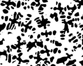
The thresholded white features in the Dendrite image
However, if the features are being measured as well as counted, features that touch any edge cannot be included (because they cannot be measured). Large features are more likely than small ones to be affected. The adjusted or effective count takes into consideration the probability that other features of the same size and shape would touch an edge and have to be rejected. The adjusted count for each feature is calculated from the feature dimensions, listed in the comprehensive output of feature measurements, and used when “Edge Correction” is selected in IP•Measure Features–>Plot (Distribution) . Note in particular the different total counts, mean values, and shapes of the distribution curves.
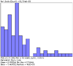
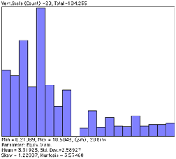
Measurements on the Dendrites image without and with correction for edge-touching features.
The next example shows a typical sequence in which some processing is required prior to measurement. The image is calibrated using the micron marker (which was then erased so that it is not included in the measurement), thresholded automatically ( IP•Threshold–>BiLevel Thresholding–>Auto ), the holes filled ( IP•Morphology–>Fill Holes ), small bits of dirt and features touching two edges removed ( IP•Measure Features–>Reject Features ), watershed segmentation applied to separate the touching cells ( IP•EDM–>Watershed Segmentation ), and finally the number per unit area counted and average size determined.
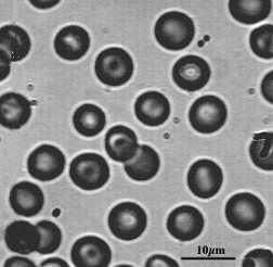
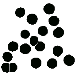
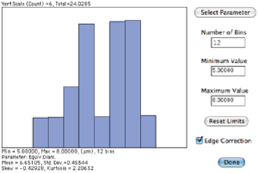
The original BloodCel image, binary result after thresholding and processing, and size measurement.