Navigation : Home : FoveaPro : FoveaPro Tutorial : Part 2
Image Analysis Cookbook 6.0: Part 2
2.A.3. Merging color channels
Grey scale images can also be combined to form a color image. This is often done when separate images of the same scene are captured with different color filters, and of course the channels may also represent non-visible colors (infrared or ultraviolet) or other signals (such as X-ray maps from the SEM). Only three images can be combined to produce a viewable image, because color space is three dimensional (ultimately this is because human vision has three kinds of color-sensitive cones in the retina), and any displayable color can be produced by combining various proportions of red, green and blue. When three grey scale images with the same dimensions are open, the Merge Channels function in the Channels window will combine them into an RGB image (you can specify which goes into which channel). When there are more than three channels, finding the most effective combination of colors is largely a trial-and-error process. Sometimes sums or ratios of individual images can be combined and displayed in a single channel. Note that Photoshop allows merging more than three channels into a “multichannel” image, which may be convenient for keeping multiple images together and is essential for principal components analysis (described in section 2.A.4), but that these cannot be displayed in meaningful colors.
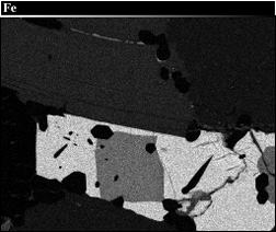
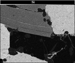
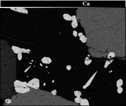
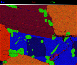
Three elemental X-ray maps and the merged RGB result ( Mica images)
Another way to efficiently combine images to produce a color composite is to insert a greyscale image into a single color channel of another image. The example shows this being done to create a stereo pair that can be viewed by using glasses with a red left eye filter and a blue or green right eye filter. Place the left eye image into the second image memory ( IP•2nd Image–>Setup ), then select the right eye image and convert it to RGB color. This is necessary in order to have color channels in which to place the other image, but initially the appearance will be unchanged because the same information will be present in all three channels. Then select IP•Color–>Transfer Channel and choose the red channel.
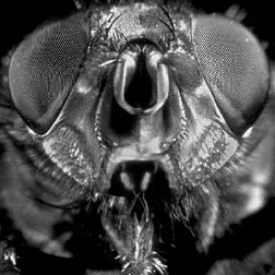
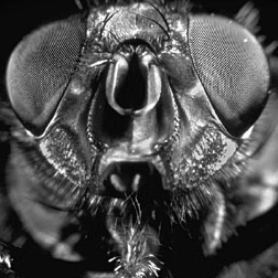
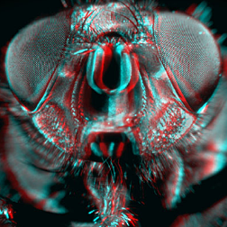
Right and left eye views and the combined stereo pair image ( FlyEye )
To illustrate fact that a color image can be interchangeably thought of as consisting of either RGB or HSI color channels, the next example uses a set of satellite images of Salt Lake City. The first three are from a moderate resolution satellite that captures separate images in visible blue, green and red. Combining them as shown above with image SaltLake_1 assigned to the blue channel, SaltLake_2 to green, and SaltLake_3 to red, produces a color image as shown (the contrast has been maximized using the IP•Adjust –> Contrast plug-in with its Auto setting; this is discussed in a following section). Another image of the same scene ( SaltLake_8 ) was acquired with a different, high resolution satellite. This image is panchromatic, covering the entire visual range of colors. Inserting it into the intensity channel of the image formed by merging the three RGB images produces a result in which the overall image sharpness is improved. Human vision judges image quality primarily by the intensity variations, and tolerates lower resolution for the color information (a fact that underlies television broadcasting and image compression). Note that the original color image was created by merging RGB channels but is then treated as an HSI image to replace the intensity channel. The conversion between these color spaces is handled internally and automatically by the software.
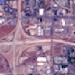

Detail of images formed with RGB channels (left) and inserting high resolution image into I channel (right)
2.A.4. Principal Components Analysis
Color images, or in fact any images containing multiple channels of data, can be analyzed using a technique known as Principle Components Analysis (PCA). This statistical method is easiest to visualize for an RGB image. Instead of the three original red, green and blue axes along which the pixel values can be plotted, PCA finds a new set of orthogonal axes rotated to align with the principal axes of the actual data. The first axis is that along which the data have the greatest scatter or dispersion, and so forth.
One use of this tool is to find the maximum contrast available in color images. As shown in the example, the staining of the tissue provides only weak visual distinction of the various cells and nuclei. The PCA technique ( IP•Multichannel –> Compute PCA Transform ) finds the most significant axes for the information and IP•Multichannel -> Apply PCA (Forward) displays those combinations of values using the red, green and blue channels to effectively separate the structures.
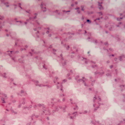
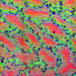
Original Turbinate image Principal components
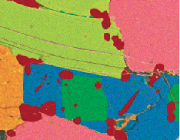 The nine SEM X-ray maps shown in 2.A.3 (Mica_Al, Ca, Fe, K, Na, O, P, Si, Ti) can only be presented in color three-at-a-time (ultimately as noted above because humans have three kinds of cones that respond to different wavelengths, and so our computer displays use three colors). With PCA it is possible to find the most significant axes in this 9-dimensional space to show the distinct compositional phases present. They appear in the display of the three most significant channels as as red, orange, yellow, green, blue and purple regions. The covariance data matrix saved to disk shows the contribution of each elemental map to the composites, and the colocalization plots show the distribution of data points on the principal planes in the PCA axes, in which the presence of the six phase clusters can be easily distinguished.
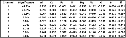
Covariance matrix for the Mica dataset
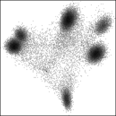
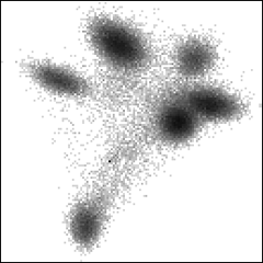
Colocalization plots of channel 1 vs 2 and 3 vs 2 for the Mica data
( IP•Multichannel->Colocalization Plots )
It is also possible to select intensity ranges in the individual channels to display the areas in the original image that they represent ( IP•Multichannel->Channel Thresholding ), or to process some of the channels in the principal components data before reconstructing the original image ( IP•Multichannel->Apply PCA (Inverse)). This latter technique can sometimes be used effectively to remove artefacts from an image, since that information is often found in the low significance channels after PCA.