Navigation : Home : FoveaPro : FoveaPro Tutorial : Part 10
Image Analysis Cookbook 6.0: Part 10
3.C. Converting texture and directionality to grey scale or color differences
In many images, structures are discernible visually based on textural rather than brightness or color differences. Processing tools such as the Sobel orientation { IP•Process –> Orientation (Sobel) } operator or a wide variety of local texture measurements based on entropy, fractal dimensions, statistical properties, etc., can convert these variations to brightness differences for measurement or thresholding. Both the range and variance operators ( IP•Rank–>Range and IP•Process–>Variance ) can be used for texture recognition purposes by using a suitably large neighborhood. In addition, the IP•Process–>Texture (Spatial) and –>Texture (Fractal) plug-ins implement several useful algorithms. The spatial algorithms are based on co-occurrence matrices and entropy calculations, while the fractal measurement uses the slope and intercept of the (log difference) vs. (log distance) data. Because the word “texture” covers such a wide range of human visual experiences, it is often necessary to try several different tools to find one appropriate to a specific application.
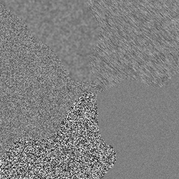
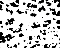
Original Texture1 image Variance (radius = 5 pixels)
Entropy (radius = 3.5 pixels) Range (radius = 4 pixels)
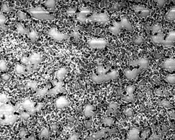
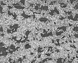
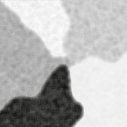
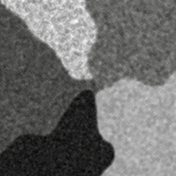
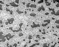
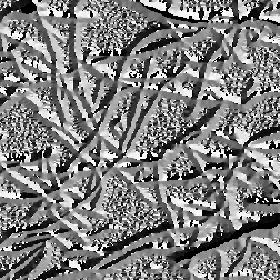
Original CurdWhey image Fractal texture intercept (radius = 5 pixels)
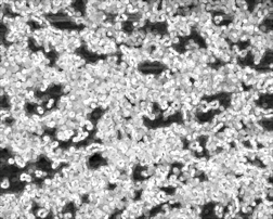
Range (radius = 2.5 pixels) Spatial contrast texture operator
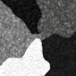
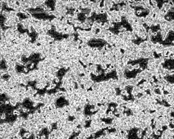
The result from using the texture operators can then be thresholded to delineate the structure of interest. In the CurdWhey example, the result of the range operator shown above was smoothed (Gaussian blur, radius = 2.5 pixels), automatically thresholded, and the result superimposed on the original image to verify the result. This was done by using the Layers capability of Photoshop, and setting the transparency of the binary image to 50%. An equivalent result can be obtained by adding the two images together.
Thresholded range image Superimposed on original CurdWhey image
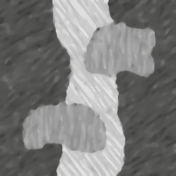
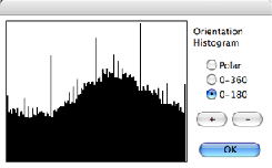
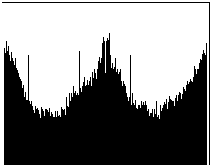
The most widely used and generally successful orientation measurement tool is based on the Sobel brightness gradient. The magnitude of this gradient was introduced above as an edge delineation tool. The angle of the vector can also be used, by assigning grey scale or color values to the angle. In the first example, the visually discernible regions in the image have the same brightness and texture but different orientations. The result of the IP•Process–>Orientation (Sobel) plug-in shows unique pairs of grey scale values in each region, which represent 180 degree differences in vector orientation (and thus are 128 grey scale values apart). This image can be thresholded most easily after applying a color table (FoldGrey.act) that duplicates the grey values assigned to the 0-180 and 180-360 degree range, as shown. In the example, the three well-separated peaks in the histogram correspond to the three region orientations in the original image. The horizontal axes covers the range from 0 to 180 degrees.
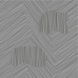
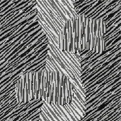
Original Texture2 image Orientation operator applied
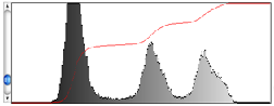
FoldGrey CLUT applied and median filtered Histogram showing three distinct peaks
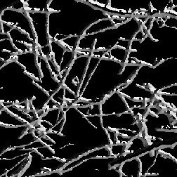
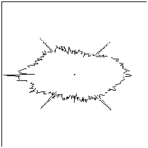
The orientation of fibers, scratches or other similar structures can be directly measured by using the histogram of the image that results from the application of the orientation filter. In the example, the relative length of curved fibers having each orientation is revealed by the corresponding number of pixels recorded in the histogram, which for convenience of interpretation is plotted as a rose plot. The preferred orientation of the fibers is immediately apparent. (The spikes at multiples of 45° are an artefact of the procedure that may be useful for inspection of the plots.)
Original Collagen image (fragment) Orientation operator applied
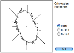
Histograms of the orientation image: left - 0-180 degree linear plot, right - rose plot
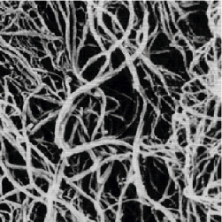
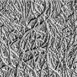
If the fibers do not cover the entire image, it is necessary to restrict the measurement to just the fibers. One way to do this is to duplicate the original image and threshold (as discussed in Section 4) the fibers. This image can then be applied as a mask to the orientation image as shown in the example, setting all of the pixels in the background to black. The procedure is to place the binary image into the second image memory ( IP•2nd Image–>Setup ), select the orientation image, and use the IP•Math–>Keep Darker Values routine.
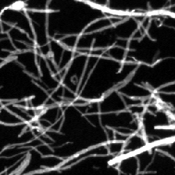
Original Fibers image (fragment) Orientation result
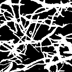
Thresholded binary image of background Combination of orientation and binary images
Histograms showing the fiber orientation: left - 0-360 degree linear plot, right - rose plot
Another useful way to represent the orientation information is to assign colors to the grey scale values, since the hue values around the color wheel can effectively represent angles. In the example shown, the edges in the original image are first outlined ( IP•Process–>Find Edges–>Sobel , followed by inverting the image with Image–>Adjustments–>Invert to make the edges bright). This image is then converted to RGB mode so that it can display color ( Image–>Mode–>RGB Color ). Then the orientation operator ( IP•Process–>Orientation ) is applied to a second copy of the image. These angle values are then transferred to the hue channel of the edge image, by first placing the orientation image into the second image memory ( IP•2nd Image–>Setup ) and then selecting the edge image and choosing IP•Color–>Transfer Channel–>Hue . The colors associated with each orientation angle of the edges (or any other structure) are made visually apparent.
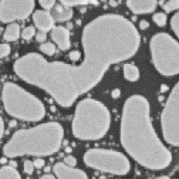
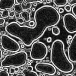
Original Au_Resn image (fragment) Edges delineated
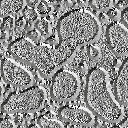
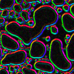
Angle values calculated Angle values assigned to the hue channel