Navigation : Home : FoveaPro : FoveaPro Tutorial : Part 8
Image Analysis Cookbook 6.0: Part 8
3.A.2. Sharpening (high pass filters)
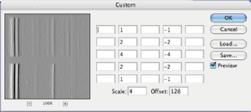
Fine detail with a known orientation can be enhanced by a derivative, an example of a convolution kernel that is neither symmetrical nor positive like the Gaussian smooth shown in Section 2.B.1. The example shows the construction of the kernel with the Filter–>Other–>Custom function. Notice that the kernel takes the difference in the horizontal direction but performs averaging in the vertical direction to reduce noise. Also, the offset factor produces a medium grey where there is a zero difference, so that positive and negative values can be seen. The scale value is typically set equal to the largest factor in the kernel or to the sum of positive values, to keep the values within range. The IP•Process–>Custom plug-in is similar but allows entry of real numbers (vs. integers), a larger array, and selection of autoscaling.
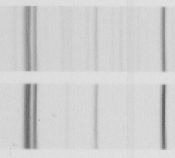
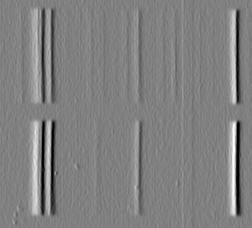
Original Debye image (fragment) and the result of the horizontal derivative filter
The directional derivative is sometimes called an “embossing” filter because it gives the visual impression of shadowed surface relief. One use of this filter is to eliminate directional noise or shadows in an image by orienting the derivative parallel to the orientation of the marks. In the examples, the markings on the surface of rolled metal interfere with the ability to see the grain structure, and the shadows interfere with the ability to see footprints in the snow. Using the Photoshop Filter–>Stylize–>Emboss routine allows setting the direction to match the marks and thus eliminate them.
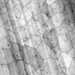
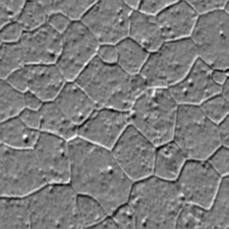
Original Extrusn image, and the result of setting the embossing filter to a direction of 110 degrees
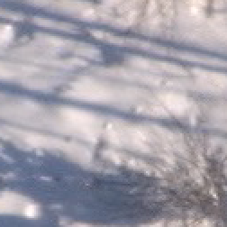
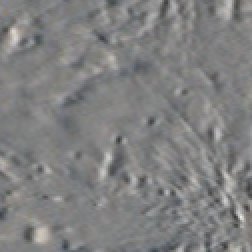
Original Footprints image (fragment), and the result of embossing at an angle of 167 degrees
Changing the orientation of the derivative affects detail with the corresponding directionality. In order to enhance detail that may have any orientation in the image, a second derivative (Laplacian) can be used instead of a first derivative. The Laplacian result is often added back to the original image (which can be done by increasing the weight for the central pixel by 1) to provide a more readily interpretable image. This is often called a “sharpening” filter; the offset value used in the directional derivative and Laplacian is omitted for the sharpening filter. The 3x3 kernels of weights are shown in the examples. Classical sharpening operations increase the local contrast at fine detail and are equivalent to FFT-based high-pass filters as illustrated in Section 2.B.3.
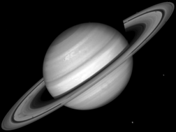
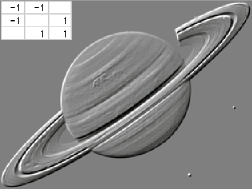
Original Saturn image Directional Derivative
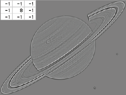
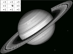
Laplacian Sharpening filter
3.A.3. Unsharp mask and difference of Gaussians
The sharpening filter shown above compares each pixel to its immediate neighboring pixels. The unsharp mask is a more general version of the same idea, and is a powerful tool derived from long-established photographic darkroom technique. A copy of the image is blurred, typically with a Gaussian filter large enough to remove whatever important detail is present. This is then subtracted from the original, since the difference is that same detail. In the built-in Photoshop unsharp mask ( Filter–>Sharpen–>Unsharp Mask ), an adjustable percentage of this difference (the detail) is added back to the original.
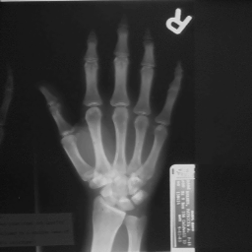
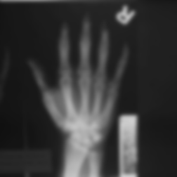
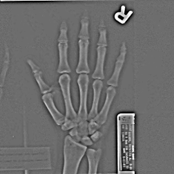
Original Hand image Gaussian blur (2.5 pixel radius)
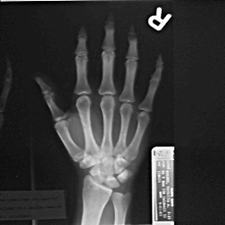
Subtracting blur from original Added back to original
These sharpening methods increase the visibility of noise, so the Difference of Gaussians (DoG) technique, equivalent to a band-pass filter in Fourier space, is a better choice for noisy images. This uses two blurred copies of the original image, one with a small standard deviation that removes the high frequency noise, a second that removes the detail (as well as the noise). The difference shows edges while suppressing the effects of the noise. The IP•Process–>Difference of Gaussians plug-in allows setting the two smoothing values (one is typically about 3-7 times larger than the other).
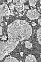
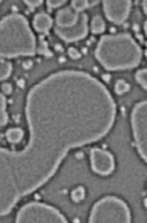
Original Au_Resn image, sharpening filter and difference of Gaussians
3.A.4. Color images should be processed in HSI space
Working on the separate RGB channels produces different ratios of values that are perceived as extreme color noise. The plug-ins automatically convert to HSI space and operate on just the intensity channel. In Photoshop, it is equivalent to change the image mode to Lab, and select just the L channel for processing.
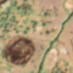
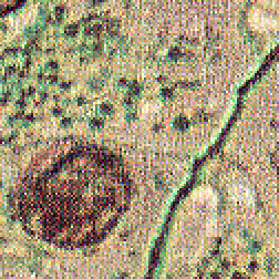
Original Tissue1 image (fragment) 3x3 sharpening filter applied to RGB channels
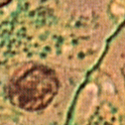
Difference of Gaussians filter applied to intensity channel only
3.A.5. Feature selection based on size
The difference of Gaussians compares the value of a small central neighborhood to the surrounding neighborhood. A different approach uses two different neighborhood sizes but compares the ranked maximum or minimum values. The top hat filter ( IP•Rank–>Top Hat ) can be used to select bright or dark objects for retention or removal (in the latter case it is called a rolling ball filter). As shown in the diagram, features that are too large for the central region are ignored by the filter. Features that fit into the smaller interior neighborhood (the crown of the hat) and are separated by the difference between the two neighborhood sizes (the width of the brim of the hat) are selected. The result of the top hat filter is a medium grey value except where features are found, where the difference between the brightest (or darkest) pixel value in the interior region and the brim is suitable for thresholding.
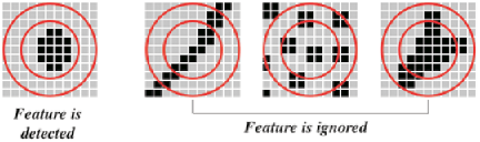
Principle of the top-hat filter: the darkest (or lightest) value in the interior region
is compared to that in the surrounding annulus and the difference retained.
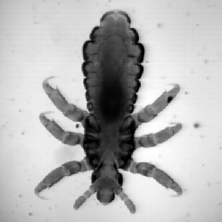
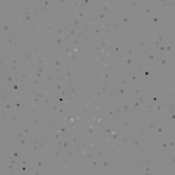
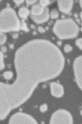
Original Bug image and the result of the top hat filter, which finds the dust particles on the slide
The top hat filter is particularly useful for locating peaks (“spikes”) in FFT power spectra. In the example, this is used to remove periodic noise automatically instead of the manual marking of spikes shown in Section 2.B.3. Thresholding the top hat for the dark spots, inverting the resulting binary image to remove the selected frequencies, and filling the central spot (which represents the mean brightness of the image) produces a mask that can be used with the inverse Fourier transform to produce the image without the periodic noise.
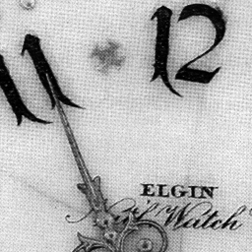
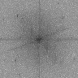
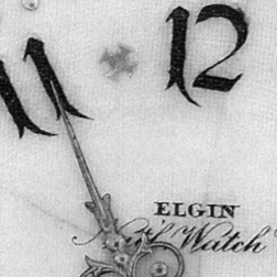
Original Clock image and its Fourier transform power spectrum
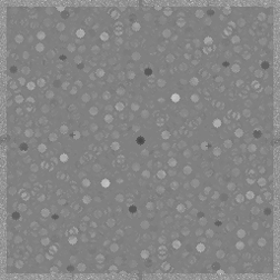
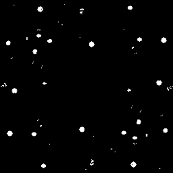
Application of the top hat filter to the power spectrum, and the mask that eliminates the noise frequencies
Inverse FFT using the mask removes the periodic noise
The same procedure can be used to keep periodic structure and eliminate random noise, as shown in the example in Section 3.D.1, below. This is an effective way of averaging together all of the repetitions of the same structure in the original image.