Navigation : Home : FoveaPro : FoveaPro Tutorial : Part 7
Image Analysis Cookbook 6.0: Part 7
2.F. Focus problems
2.F.1. Shallow depth of field
When the optical depth of field is insufficient to produce an image in which everything is in focus, it may be practical to capture a series of images and combine them. This method requires that the images be aligned and at the same magnification scale. That is difficult to do when the focus is adjusted by altering the lens (as on a typical camera). Multiple images obtained by moving the lens relative to the sample (as is done in a typical light microscope) can be combined by keeping the in-focus pixels from each. Place one image into memory ( IP•2nd Image–>Setup ), select the next image and choose IP•Adjust–>Best Focus . Repeat this for each of the images in the series.
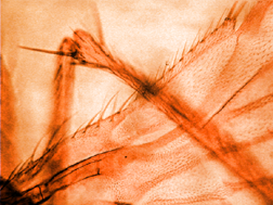
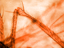
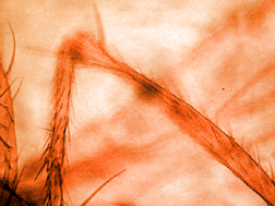
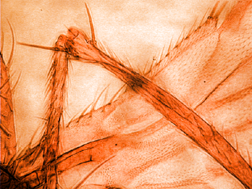
Three light microscope images ( Fly_1,2,3 ) taken by raising the stage to bring different
regions into focus, and the composite in which all regions are in focus.
2.F.2. Deconvolution of blurred focus
The usual causes of blurred images are out-of-focus optical settings or camera motion. It is possible to correct a significant portion of these sources of blur provided that the same cause of blur affects the entire scene. The point-spread function (PSF) is an image of the blur applied to a single point. If the PSF can be directly recorded, for instance in astronomy as the image of a single bright star, then in the ideal case, dividing the Fourier transform of the PSF into the transform of the blurred image, and performing an inverse FFT back to the pixel domain, recovers the unblurred image. In the typical real case, the presence of noise in either image limits the amount of deconvolution that is possible, and the Wiener constant is introduced to limit the effect of the noise.
In the case in which a point spread function has been measured, place the PSF image into memory ( IP•2nd Image –>Setup ), select the blurred image, and choose IP•FFT–>Deconvolution . Either apodization (ignoring terms in the transform where the denominator in the division gets too small) or an adjustable Wiener constant (controlling the tradeoff between sharpness and noise) can be selected. The Fourier transforms and other computations are performed automatically, and the images are not restricted to power-of-two dimensions (they are padded automatically to the next larger size).
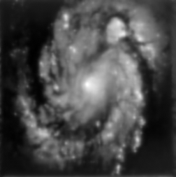
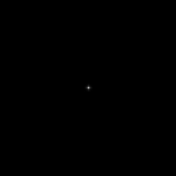
Original Hub_blur image and the measured point spread function ( Hub_psf )
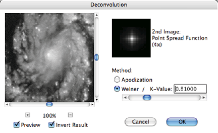
Dialog for the deconvolution plug-in
When no measured PSF is available, it may still be possible to perform a useful deconvolution to remove blur by interactively modeling a plausible point-spread function. Typically a Gaussian shape provides a good approximation to out-of-focus optics, while a straight line segment models blur due to motion. Adjusting the length and angle of the line (and perhaps its blur), or the standard deviation of the Gaussian (and perhaps the amount and orientation of any astigmatism) can often be done efficiently while watching the results in a preview. The example shows removal of motion blur from an aerial photograph (the line shown for the PSF corresponds to the motion of the airplane during the exposure) using the IP•FFT –> Interactive Deconvolution plug-in. Notice that the deconvolution is imperfect at the top and bottom of the image, because the motion included a slight component of rotation as well as translation.
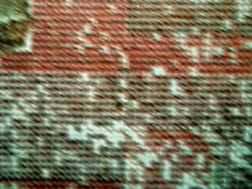
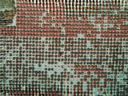
The original Orch_Blur image and the result of interactive deconvolution
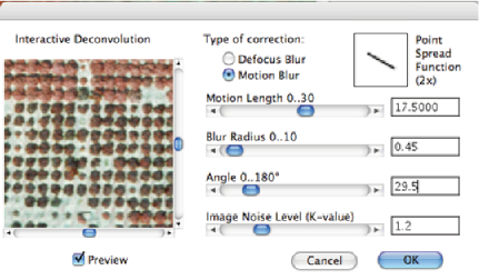
Dialog for the interactive deconvolution plug-in
2.G. Tiling large images
2.G.1. Shift and align multiple fields of view
One way to obtain a high resolution image of a large field is to capture a series of images and “stitch” or “tile” them together to make a single large picture. When this is done for panoramic imaging, with a camera mounted on a tripod, it is usually necessary to overlap the images and often to make local scale adjustments so that they fit together properly. But for situations such as a microscope in which image distortions are minimal and stage motion can be controlled, it is often practical to combine multiple tiles simply by creating a large enough space (choose one image and use the Image–>Canvas Size adjustment), and then copy and paste each image in place. Since the images are pasted into separate layers initially, they can be shifted for proper alignment (the arrow keys are useful for single-pixel shifts, the IP•Adjust–>Nudge function for fractional pixel adjustments). Layers can be shown or hidden on the display by clicking on the “eye” icon for each, or the layer opacity adjusted, to facilitate viewing and comparison. When all of the tiles are positioned correctly, the Layer–>Flatten Layers selection combines them into a single image. The Photoshop File–>Automate–> Photomerge function can assist in this process. There are also third-party plug-ins and stand-alone programs that perform this function.
3. Enhancement of image detail
Many of the same classes of tools described above can also be used to enhance the visibility of some of the information present in the image, usually by suppressing other types of information (such as increasing local contrast by suppressing global intensity variations). The purpose may either be to improve visual interpretation of images (including better pictures for publication), to facilitate printing of images, or to allow subsequent thresholding of the image for measurement purposes.
3.A. Poor local contrast and faint boundaries or detail
3.A.1. Local equalization
Increasing the local contrast within a moving neighborhood is a powerful non-linear tool for improving the visibility of detail. Local contrast equalization and variance equalization ( IP•Process–>Local Equalization ) suppress overall contrast while revealing local detail. Variance equalization is somewhat better at rejecting noise, but all local enhancement methods will also increase noise visibility which is why the processing steps in Section 2 should be used before those in Section 3. Adaptive equalization ( IP•Process–>Adaptive Equalization ) provides additional flexibility for making detail visible, as shown in the examples. Note that combining the results of this enhancement with surface rendering (discussed below) is particularly effective. For color images it is important to process the data in hue-saturation-intensity space (all of the plug-ins do that automatically, or you can convert to Lab space and process just the Luminance channel).
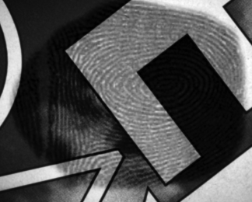
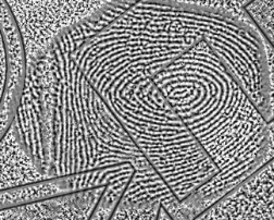
Original FingerP2 image and the result of local contrast equalization
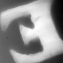
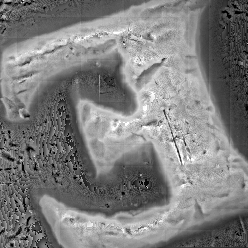
Original CoinSurf image and the result of local variance equalization
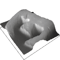
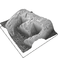
Rendered CoinSurf data as an surface display, and with the equalized image applied to the surface.
The surface rendering plug-ins ( IP•Surface Processing –> Plot 2nd as Surface and
–> Reconstruct Surface with Overlay ) are discussed in section 3.A.6
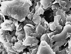
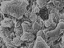
Original SEM image ( Contrast2 ) and the adaptive equalization result
Showing enhanced detail on the surface and in the cavity
Images that have a high dynamic range, such as medical X-rays, and scenes that include brightly lit areas and deep shadow, typically require processing to compress the overall contrast range while preserving or enhancing the local detail. A combination of high pass filtering (performed in either the spatial or Fourier domains) and histogram shaping are often used as shown in the example.
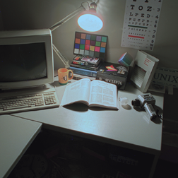
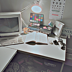
Original Desk image and the result of filtering and histogram shaping.