Navigation : Home : FoveaPro : FoveaPro Tutorial : Part 5
Image Analysis Cookbook 6.0: Part 5
2.C. Nonuniform image illumination
2.C.1. Is a separate background image available?
Nonuniform lighting, optical vignetting, fixed patterns in the camera response, or other factors can cause image brightness or contrast to vary from side to side or center to edge, so that the same feature would appear to have different brightness (or color) depending on where it was located. If these factors remain constant over time, one practical solution is to capture a separate background image using identical settings but with no sample present (such as a photograph of a neutral grey card on a copy stand, a blank slide in a light microscope, or a clean stub in the SEM). This image can then be used to remove the nonuniformities from acquired images by either subtraction or division. The choice of subtraction or division depends on whether the camera response in logarithmic (subtraction) or linear (division). Photographic film, video cameras, and some digital cameras are logarithmic in output vs. light intensity, while scanners and CCD detectors are inherently linear (division). Sometimes the only good way is to try both and see which produces a flat response.
In the example shown, a background image was acquired with the same lighting conditions as when the sample was present, and then subtracted to remove the nonuniformity due to placement of the lamps. The subtraction procedure is to place the background image into the second image buffer ( IP•2nd Image –> Setup ), select the image of interest, and then choose IP•Math –> Subtract .
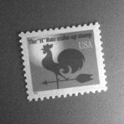
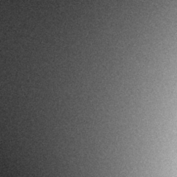
Original image ( Lighting1 ) and the corresponding background with the feature removed ( Lighting2 )
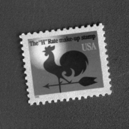
Subtracted (leveled) result.
Unfortunately, in many cases a suitable background image can not be (or was not) acquired, or there are effects due to the specimen itself (variations in thickness or density, surface curvature, etc.) that cause nonuniformities in the image. In these cases, several other methods are available. Sometimes there are enough areas of a uniform background available in the image to construct a background mathematically. One method for doing this is to manually select the background areas (for instance with the Photoshop marquee or lasso tools, or the wand tool) and then choose IP•Adjust–>Background Fitting . That uses all of the points in the selected area (which should be distributed across the image, not all in one corner!) to fit a polynomial function. Then removing the selection or selecting the entire image and choosing IP•Adjust–>Background Removal subtracts the constructed polynomial from the image. The polynomial is remembered and will be used again until a new one is established.
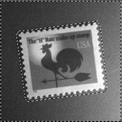
Selecting the background areas to construct a polynomial background, and the result of removing it.
2.C.2. Is background visible throughout the image?
Leveling based on fitting a polynomial can be applied automatically if the background regions are either lighter or darker than the features (and of course provided that representative background patches are well distributed across the image). The IP•Adjust–>AutoLevel functions divide the image up into a grid and find the brightest (or darkest) pixel values in each segment, and then construct the polynomial and subtract it. This is a very rapid and effective tool in many cases. In the example shown, the presence of the nonuniform lighting (due to optical vignetting) is made more visually evident by using false color or pseudo color to assign a rainbow of colors to the grey scale values (convert the image mode to RGB color and use the IP•Color–>Apply Color Table plug-in to load the desired color scale).
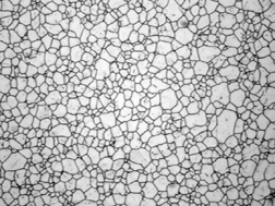
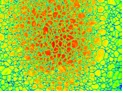
Original Gr_Steel image with vignetting False color used to show brightness variation
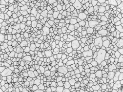
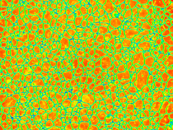
The same image after automatic leveling to make all of the bright values uniform
2.C.3. Correcting varying contrast across an image
The polynomial method can be extended to fit both the brightest and darkest values across the image in order to compensate for variations in contrast, for example due to thickness changes in samples viewed in transmission. In the example, it was necessary to first reduce the speckle noise using a median filter before using IP•Adjust–>AutoLevel plug-in to level the contrast in the image. The local contrast is stretched linearly between the brightest and darkest curves.
Original Shading1 image After median filter and autoleveling contrast
2.C.4. Are the features small in one dimension?
The polynomial leveling method works well when lighting or vignetting cause a gradual variation of brightness with position. An irregular pattern of variation, for instance due to surface geometry or local density variations, can be more effectively corrected using rank-based leveling to remove the features and leave just the background, for subsequent subtraction or division. The median filter introduced above as a noise removal technique is one example of rank filtering. Instead of replacing each pixel with the median of the values in a small neighborhood, it is also possible to choose the brightest or darkest value. Section 5.A. on morphology illustrates several ways that erosion, dilation, openings and closings are applied to images (a more general discussion of morphological processing is presented in a later section). One of those methods operates on grey scale images. In the first example shown, replacing each pixel with its darkest neighbor (grey scale dilation) removes the features to produce a background which is then subtracted to level the overall contrast. If the features had been dark on a light background, they would have been removed with a grey scale erosion. These operations are selected in the IP•Rank–>Grey Scale Morphology dialog.
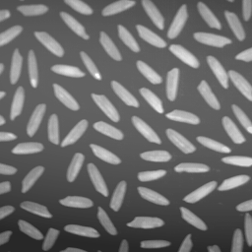
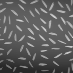
Original Rice image One iteration of grey scale dilation

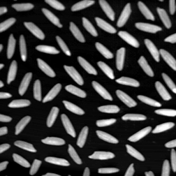
After four iterations the rice grains are removed Subtracting the background from the original
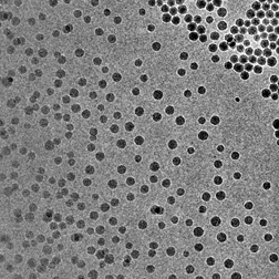
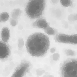
This method is made more general by combining erosions and dilations to preserve the sizes of the background structures. In the next example, in which the background density varies because of stained organelles, the small dark gold particles are removed by grey scale erosion but this also shrinks the organelles. Following two iterations of erosion, two iterations of dilation are used to restore the organelle size, and then the resulting background is divided into the original to leave just an image of the gold particles. The sequence of erosion followed by dilation is called an opening. The opposite sequence of dilation followed by erosion is called a closing. Either can be selected as single step operations in the IP•Rank–>Grey Scale Morphology dialog.
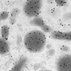
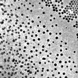
Original Gold2 image After two iterations of erosion
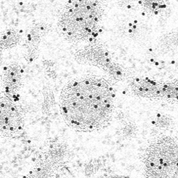
After two iterations of dilation (opening) Dividing the background into the original
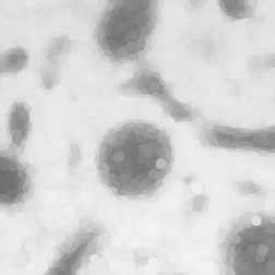
This technique can also be applied to color images. The IP•Rank–>Color Morphology routine performs erosion, dilations, openings and closings based on color. Select the color (in the example shown, the red of the blood vessels) with the eyedropper tool, so that it becomes the foreground color in the tool palette. Then select the plug-in. In the example, an opening (erosion followed by dilation) of the red color was used to remove the blood vessels, and the resulting background was then subtracted from the original to remove the variation in brightness and color leaving just the blood vessels. It is sometimes useful to blur the background produced by the morphology routines (e.g., using a Gaussian blur) before subtracting or dividing, to eliminate contours (this was done in the example shown).
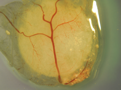
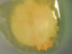
Original Yolk image After opening and Gaussian blur
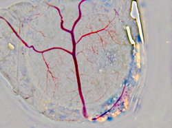
After subtraction of the background