Navigation : Home : FoveaPro : FoveaPro Tutorial : Part 15
Image Analysis Cookbook 6.0: Part 15
5. Binary image processing
5. A. Removing extraneous lines, points or other features
5.A.1. Erosion/dilation with appropriate coefficients to remove lines or points
The use of combinations of erosion, dilation, opening and closing permit selective correction of binary image detail when thresholding leaves artefacts behind. Classical erosion and dilation are morphological operators that compare pixels to their immediate neighbors to determine whether to change black to white or vise versa. An opening is the sequence of erosion followed by dilation, while a closing is the opposite.
The IP•Morphology–>Classic Morphology plug-in provides two parameters to control the processes of erosion, dilation, opening and closing: The number of iterations of adding and/or removing pixels is related to the dimension of the modification. The coefficient is a test parameter that the number of adjacent neighbor pixels (out of the 8 possible) that are opposite in color (black or white) to the central pixel must exceed for it to change.
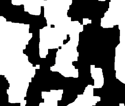
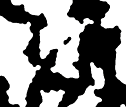
The Panda test image is a useful example to explore the consequences and uses of the various settings. For example, an erosion with a coefficient of 7 will remove only isolated single pixels without affecting anything else, while an opening with a coefficient of 1 will remove the fine lines and a closing will fill small gaps to connect the leaves to the branches. A coefficient of 0 (zero) corresponds to the traditional meaning of erosion and dilation, changing the color of any pixels that touch any neighbors of the opposite color. That is, in traditional erosion any white pixel adjacent to a black one becomes black , while in traditional erosion any black pixel adjacent to a white one becomes white .


Original Panda image Erosion, Coefficient = 7


Opening, Coefficient = 1 Closing, Coefficient = 1
5.A.2. EDM based morphology to remove small features or protrusions, and fill in gaps
Classical erosion and dilation alter shapes when the number of iterations is large. Erosion and dilation based on the Euclidean distance map are much faster operations, and more isotropic than classical pixel-based techniques. The distance map assigns values to pixels within features that measure the distance to the nearest background point and thresholds the result. Eroding or dilating the example circle with IP• Morphology –>EDM Morphology produces circles of larger or smaller size without the distortions produced by the classical neighboring-pixel technique. In the illustrations below, Photoshop layers have been used with partial transparency to show the results of 25 iterations or erosion and dilation of the original circle, comparing the classical iterative method with the EDM technique. Notice also that the classical technique produces results of different size with the same number of iterations, depending on the neighbor test coefficient.

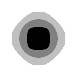
Coefficient = 0 Coefficient = 1
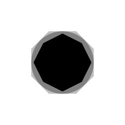

Coefficient = 3 EDM-based results
Closings and openings can be used in combination to clean up images after thresholding, as shown in the example below. The structures of interest are the region with the lamellar plates and the single-phase region without the lamellae, but simple thresholding only delineates the lamellae. Filling the spaces between the lamellae with a closing, and then removing the isolated dark spots with an opening, produces the desired image of the regions. Doing this with classical morphology (coefficient = 0, closing with 6 iterations and opening with 4) produces boundaries that have preferred directions, while EDM-based morphology (distance of 5.5 pixels) produces a more realistic result. Note that while classical erosion and dilation is limited to an integer for the number of iterations, the EDM method accepts real numbers since the distance of each pixel from the boundary is measured exactly.
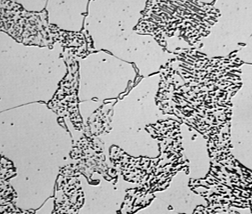
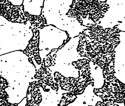
Original Pearlite image Thresholded binary
Classical closing and opening EDM-based closing and opening
To minimize confusion, be aware that there are four “morphology” plug-ins provided, each useful for different situations. IP•Morphology–>Classic Morphology is used only for binary (black and white) images and counts the immediate neighbor pixels that are different from the central pixel to determine its fate. It is most useful for removing lines and points by controlling the coefficient, and is best used with a small number of iterations. IP• Morphology –>EDM Morphology is also applied to black and white images, and uses the Euclidean distance map to determine distances. It produces the most isotropic results when large distances are needed. IP•Rank–>Grey Scale Morphology replaces the central pixel by its brightest or darkest neighbor, and is used for a variety of operations on grey scale images. If applied to a binary image, it is equivalent to classic morphology with a coefficient of 0. IP•Rank–>Color Morphology replaces the central pixel by the neighbor that is most like or unlike the current foreground color, and is used on color images.
5.B. Separating features that touch
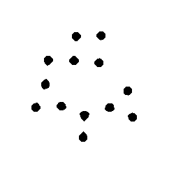
The watershed, based on the EDM, is a powerful tool for separating touching convex shapes. The method is useful for section images and surface images in which features are adjacent. If there is slight overlap, the feature shapes may be altered due to the overlapping portion being cut off. If the overlap is too great the method will fail, and in three-dimensional samples, small features may be hidden by large ones.
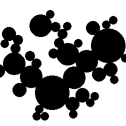
Original Circ_Mix image (fragment) IP• Morphology –>Watershed Segmentation result
It is often useful to verify the results of thresholding and segmentation by overlaying the result on the original grey scale or color image. This is easily done using Photoshop layers. In the example the outlines of the watershed-segmented particles are superimposed on the original.
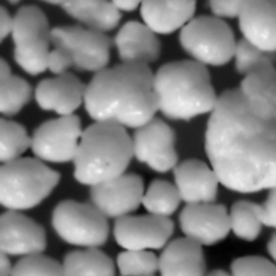

Original Sand image Thresholded
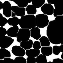
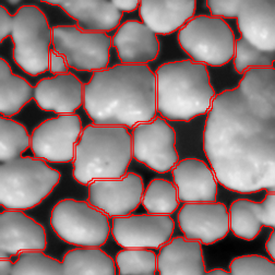
Watershed Outlines superimposed on original
The watershed method fails when the touching features contain holes, as shown in the example below. However, in this case it is possible to distinguish the holes within the features (which are fairly round) from those between the features (which are not) by measurement. The procedure is to measure the holes as features (Section 6.E), select the round ones (Section 6.F), combine (Boolean OR, Section 5.C) those with the original thresholded image, and then perform a successful watershed segmentation of the cells.
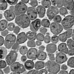
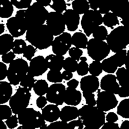
Original Cells image Thresholded
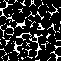
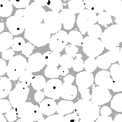
Unsuccessful watershed attempt Measuring the holes (dark ones are kept based on shape)
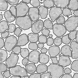
Combining the round holes with the original binary Watershed segmentation (shown as outlines)
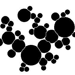
Alternative but less commonly used methods rely on successive erosions to separate features. For example, eroding the circles in the example shown until they separate, then skeletonizing (discussed in Section 5.D.1 below) the background and erasing those lines from the original separates the features. However, this approach would not work for the Circ_Mix image above because the range of sizes would result in the removal of some features before others separate.

Original Circles image Eroded until features separate
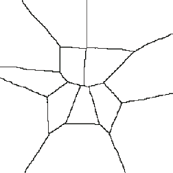
Skeleton of the background Removal of the skeleton lines from the original
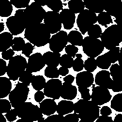
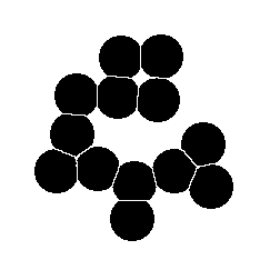
Another technique that is sometimes used to determine a distribution of particle sizes employs grey scale erosion or dilation (see Section 2.C.4). In the example shown, replacing each pixel by its darkest neighbor (grey-scale dilation) reduces the size of features and eventually causes them to disappear. Thresholding the image at each stage and counting the number that disappear (which requires some Boolean logic that is described below) provides a measure of the number of particles with a radius equal to the corresponding number of erosions, and allows a size distribution to be constructed. The assumptions in this method are that the particles separate before they disappear, and that they are sufficiently round that the radius measurement obtained from the number of iterations adequately describes their size.
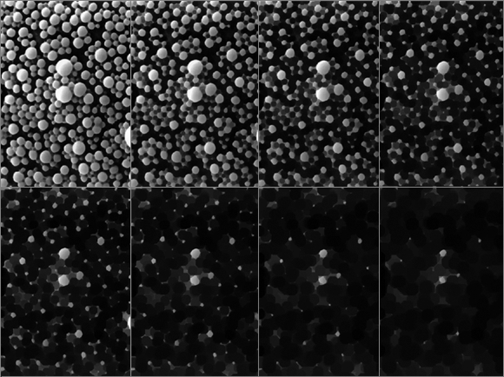
Sequence of grey scale dilations applied to the Lipid image (fragment)
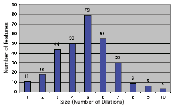
The resulting size distribution plot for the particles