Navigation : Home : FoveaPro : FoveaPro Tutorial : Part 11
Image Analysis Cookbook 6.0: Part 11
3.D. Fourier-space processing
3.D.1. Isolating periodic structures or signals
The FFT power spectrum can facilitate the selection of regular structures in the image and their measurement. Besides its use for removing periodic noise from images (e.g., electronic interference, vibration, or halftone printing patterns), this facilitates averaging and measuring repetitive structures (e.g., TEM images of atomic lattices). Note that the FFT routine used in the plug-ins requires images to have dimensions that are a power of 2 (256, 512, ...). For images of other sizes, either create a square ROI of these dimensions within the image (set Style = Fixed Size), or enlarge the canvas size ( Image–>Canvas Size )
The same procedure illustrated in Section 3.A.5 above can be used to keep periodic structure and eliminate random noise, as shown in the following example. This is an effective way of averaging together all of the repetitions of the same structure in the original image. The top hat filter was used to automatically locate all of the spikes in the FFT power spectrum of the original image, and thresholded to create a mask or filter that keeps those frequencies and eliminates others.
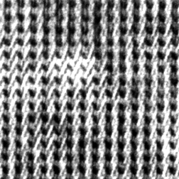
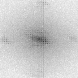
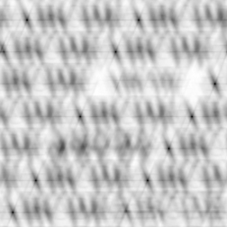
Original Mullite image and its FFT power spectrum
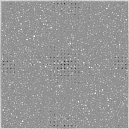
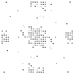
Application of a top hat filter to the power spectrum, and a mask that keeps the periodic frequencies
Result of using the mask with an inverse FFT
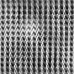
Measurement of spacings can also be performed directly with the power spectrum. As shown in the example, the lowest frequency (smallest radius) spike in the Fourier transform of the muscle image corresponds to the spacing of the z bands (spikes at multiples of this frequency are related to the shape of the bands’ intensity profiles). This radius can be converted directly to the spacing (equal to the image width divided by the radius) using the IP•FFT–>Show Fourier Values function. If the original image had been calibrated in µm, as shown in Section 6.A.1, the value would be converted rather than being shown in pixels.

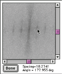
Original Muscle2 image showing z-bands Measurement of the Fourier power spectrum
3.D.2. Location of specific features
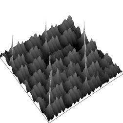
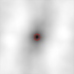
Cross-correlation with a target image is equivalent to sliding the target across the image while measuring the degree to which the pixel patterns match, and is a powerful object finder. The example illustrates the procedure. A target image is placed in the second image memory ( IP•2nd Image–>Setup ), and then the image of interest is selected and the IP•Fourier–>Cross Correlation function chosen. The two images do not need to be the same size (and are not restricted to the power-of-two dimensions required by the forward and inverse FFT plug-ins). The resulting image has spikes that locate the features similar in shape and contrast to the target, and this can be thresholded, or a top hat filter applied as required. The surface rendering shows why these are called “spikes.”
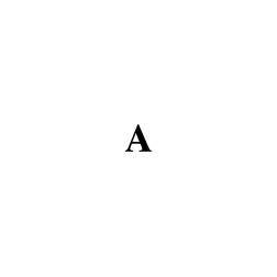
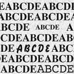
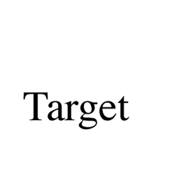
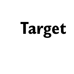
The target image ( Text_2 ) and the image to be searched for the same shape ( Text_1 )
Cross-correlation result marking the location of the target shape
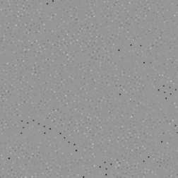
The next example shows a more realistic application, the counting of particles that are partially dispersed on a noisy background (a Nuclepore filter). There is also debris present, and particles adjacent to others are different in brightness than isolated ones. Manual selection of several representative particles and averaging their images together produces a suitable target. Cross-correlation and a top hat filter locate each of the particles, so that thresholding and counting ( IP•Measure Features–>Count ) can be performed. If the thresholded image of the particle locations is then convolved with the original target ( IP•Fourier–>Convolution ), an image showing the particles without the background or debris is obtained.
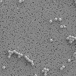
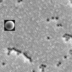
Original Count1 image The averaged target image (inset) and the cross-correlation result
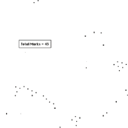
Application of a top hat filter Thresholding and counting
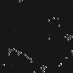
Convolution
If the same image is used for the target image and the cross-correlation image, the result is auto-correlation. This result can be best understood as imagining sliding an image across itself and seeing how far it must be displaced before features no longer lie on themselves. Hence, auto-correlation provides dimension information on the structuring element(s) present. In the example, the small features that make up the structure are not separated and even partially hidden by others, but the auto-correlation result provides an average shape and dimension. The IP•Threshold–>Contours plug-in was used to delineate a boundary on the correlation image.
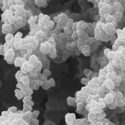
Original Cheese2 image Auto-correlation result with superimposed contour line
3.E. Other uses of correlation
3.E.1. Alignment
Cross-correlation is also used to match points in multiple images for alignment. The alignment procedure (which does not include rotation) requires placing one image into the second image memory, selecting the image to be shifted, and choosing IP•Adjust–>Align with 2nd . As shown in the example, the images do not have to match exactly. This procedure is useful before looking at image differences, lining up stereo pairs before merging or measuring them, and aligning images before combining them to form an extended focus composite.
Two images to be aligned

After alignment, a best-fit result is shown using layer transparency
A special case of alignment by shifting using cross-correlation occurs in video images. The two fields that make up one video frame consist of interlaced even and odd numbered scan lines, which are scanned 1/60th of a second apart in time. Motion of either the subject or camera can cause an offset between the two fields. The IP•Adjust–>De-Interlace plug-in finds the offset and shifts the fields for best alignment. Note that this approach is based on the assumption that the motion is uniform throughout the image or selected region.

Original Interlac image Fields aligned
The IP•Surface Measurement–>Stereo Pair Measurement routine uses cross-correlation to match regions around each pixel in the stored second image to those in the current image, and shows the horizontal displacement (proportional to the vertical elevation) as a grey scale range image.
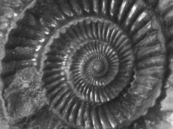
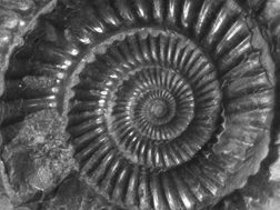
Stereo views ( Ammon_L, R )
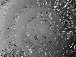
Result of stereo measurement, and the use of a median filter to remove dropouts, leveling ( IP•Surface Processing–>Flatten ) to remove the overall tilt, and contrast expansion.
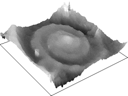
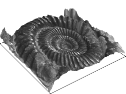
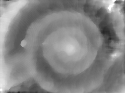
The rendered elevation measurements ( IP•Surface Processing–>Plot 2nd as Surface ), and with the original contrast superimposed ( IP•Surface Processing–>Reconstruct 2nd with Overlay )
3.E.2. Measurement of fractal dimension
The FFT power spectrum provides a direct measurement of the fractal dimension of surfaces and structures. The slope and intercept of the amplitude vs. frequency curve (on log-log axes) give the dimension and topothesy (lacunarity) as a function of direction, provided the phases are randomized.
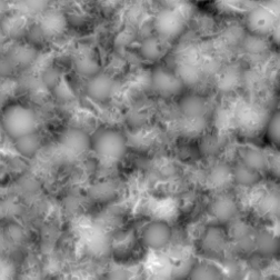
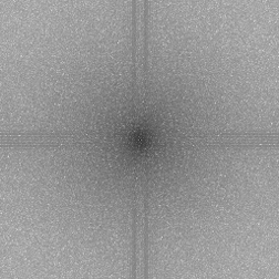
Original ShotBlas image and its Fourier transform power spectrum
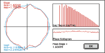
Analysis of the power spectrum showing a linear log-amplitude vs. log-frequency trend,
random phases, and isotropic intercept and slope values for the fractal.