Navigation : Home : FoveaPro : FoveaPro Tutorial : Part 18
Image Analysis Cookbook 6.0: Part 18
5.D. Feature skeletons provide important shape characterization
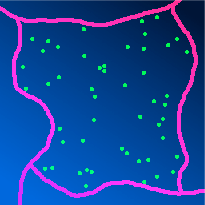
5.D.1. Grain boundary, cell wall, and fiber images
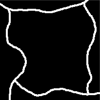
Broad thresholded lines can be thinned to single pixel width as was shown in an example in Section 4.A.2. This skeletonization is accomplished by erosion with rules that prevent removing the final line of pixels ( IP•Morphology–>Skeletonize ). Note that the skeleton is “8-connected” meaning that a pixel is assumed to touch any of its eight possible neighbors. But by this same criterion the cells or features that it divides would also be continuous, so it is often necessary to convert the skeleton to a “4-connected” line in which pixels touch only their four edge-sharing neighbors. These lines can separate the regions on either side.
End pixels in skeletons have only a single neighbor, whereas most skeleton pixels have two neighbors and those at branch points or nodes have 3 or 4. For overlapped fiber images, the number of fibers can be determined as half the number of end points, and the mean length as the total length divided by number as shown in the example. This method is also correct for structures that extend beyond the image boundaries. A single end point is interpreted as one-half of a fiber in determining an average (the other end would be counted in another field of view).
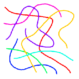
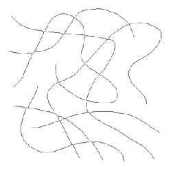
Original XFibers image Skeleton
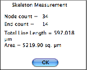
Counting the ends and measuring the length
Grain boundaries and cell walls form tessellations without end points, so pruning of branches with ends is an appropriate clean-up method. In the first example shown, the grain boundary tesselation is produced by IP•Morphology–>Pruned Skeleton .
Removal or measurement of short branches based on length also provides a powerful tool. IP•Morphology–>Skeletonize and Trim Branches was applied in the second example. Removal of branch points leaves the separate segments for measurement. The IP•Threshold–>Select Skeleton Components allows selection of any of these components. In the third example this was applied after skeletonizing to leave just the individual segments for measurement.
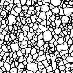
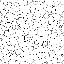
Thresholded Gr_Steel image Pruned skeleton
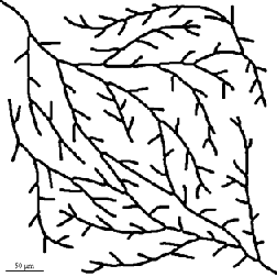
Original Branches2 image Skeleton with branches < 25 pixels removed
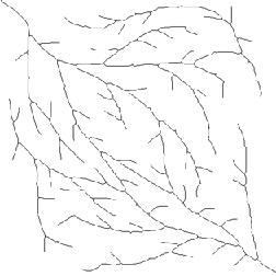
Original Root2 image Skeleton with nodes removed (fragment)
Measurement of the segment lengths
5.D.2. Measuring skeleton length, number of ends, number of branches for features
Values from skeletonized features provide basic topological (shape) information about structures, which will also be used in the discussion of feature measurement parameters. In the first example, the features are labeled with the number of skeleton end points, which measures the number of points in the original stars. In the second, the total number (43) can be counted to count the gear’s teeth. The dilated end points are superimposed on the original image using Photoshop Layers. Note: the thresholded gear image was cleaned up with an EDM-based morphological closing.
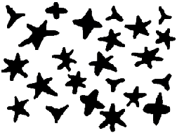
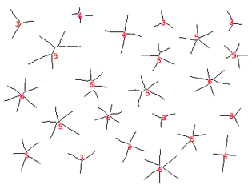
Original Stars image Skeleton and label (number of end points)
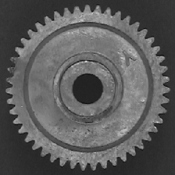
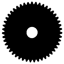
Original Gear image Binary image
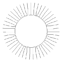
Skeleton End points superimposed on original
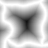
5.E. Using the Euclidean distance map for feature measurements
5.E.1. Distances from boundaries or objects
In Section 5.C.3 above, features adjacent to boundaries were selected. By assigning values from the EDM to features it is possible to select or measure features based on their distance from irregular boundaries. The assignment can be done by combining the images keeping whichever pixel is darker, or by using the binary image of the features as a mask placed on the EDM image. The EDM values can be calibrated as distance values using the density calibration routine, or just invert the EDM to measure the distance in pixels.
Original Distanc2 image Thresholded cell interior
EDM of cell interior (inverted) Thresholded features
EDM values assigned to features Measured distances from boundary
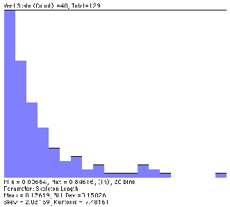
Sampling the EDM with the skeleton provides width measurement (mean, max, min, standard deviation) for irregular shapes. This method is used automatically by the feature measurement routines but can be applied manually when more complete statistics are required. Notice that the skeleton follows the central “ridge” in the EDM where the pixel values represent the radius of an inscribed circle. A histogram of the values along that ridge provides a comprehensive measurement of the feature’s width. The data are saved to disk by the IP•Measure Global–>Histogram routine and can be analyzed using Excel.

Original Width2 image Skeleton superimposed on the EDM
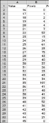
Histogram data in a spreadsheet
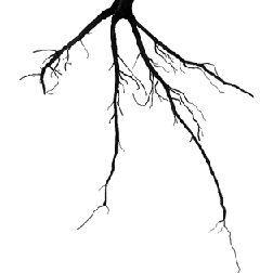
The example below illustrates the use of the EDM and skeleton together to show a complex relationship between the length of each branch and how distal it is from the cell body. The nodes are removed from the skeleton to separate the segments. Then the ends are used as markers in a feature selection operation to keep just those segments that are terminal branches. Next the EDM of the region around the cell body is generated and the values assigned to the terminal branches. Finally a plot of the length of each branch vs. the minimum brightness value (the distance of the point nearest the cell body) is constructed to show the trend. Understanding this sequence (each individual step is not shown in the illustrations) is a good indicator of mastery of these tools.
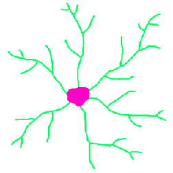
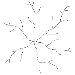
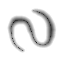
Original Neurons image Skeleton
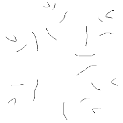
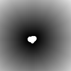
Terminal branches EDM of the region outside the cell body
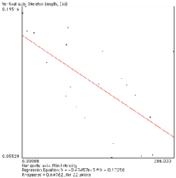
EDM values assigned to branches Plot showing shorter lengths for more distal terminal branches